Cost Functions
In my last post, I discussed how the weight (w) and bias (b) were initially chosen arbitrarily. The issue was that the line we had drawn on our graph wasn't the best fit, meaning that our model was inaccurate. This post, as well as my gradient descent post, will cover how the values of w and b can be calculated mathematically to minimize our cost.
What is cost?
Going back to my linear-regression post, we were using this graph to predict the area of a city based on its population.
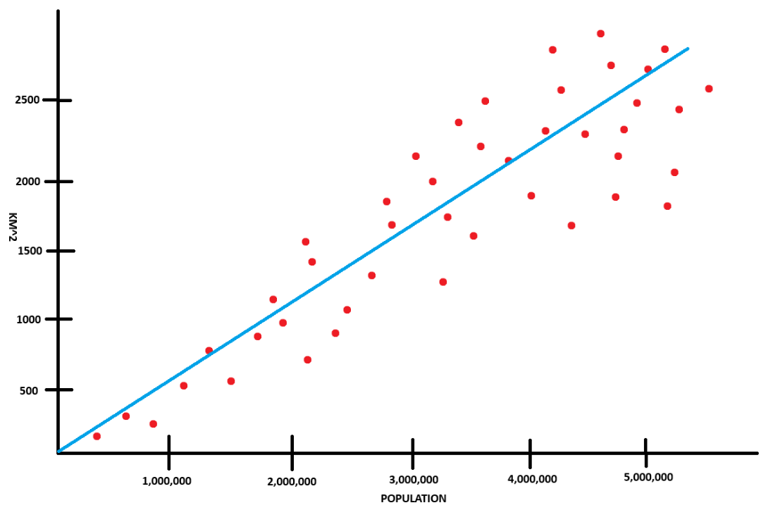
Examining it in more detail:
- x-axis: Population
- y-axis: Area
- Data points (red dots): A city's area and population
- Light blue line: Our model's predicted line
Cost is a measure of how well our model fits our data. In other words, it's the cumulative "average" of how far off our model's predictions are from the actual data points. The lower the cost, the better our model is at making accurate predictions.
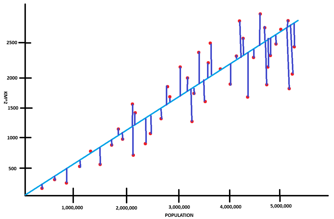
As you can see in this graph, the cost is the difference between the actual data and the predicted value which is represented by the navy blue lines.
Calculating cost
Before we jump into the cost formula, I wanted to show another method of representing the data above which could be a chart such as this one
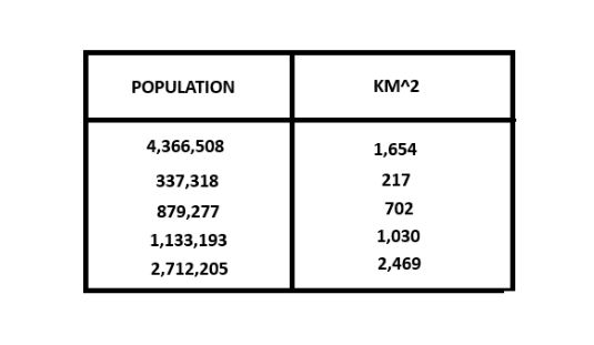
Essentially what we have are 2 arrays of data
- x (population): [4366508, 337318, 879277, 1133193, 2712205, ...]
- y (area): [1654, 217, 702, 1030, 2469...]
Then to calculate cost, we find the difference between the actual value (y) and the predicted value (fw, b(x)). In other words
- costi = (wxi + b) - yi
where wx + b is the fomula for fw,bi or our predicted value. After we calculate the cost for each item, we divide by the number of items to get the "average".
"But why is this important Gavin?" This is because the formula we'll be using, Mean Squared Error (MSE), is calculated very similarly with the only difference being that we square costi and that it has some additional notation.
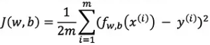
- J(w, b): The calculated cost of the current model
- m: Number of data-points
- f(x(i)): Predicted value in the ith position
- yi: Actual value in the ith position
- i: Current item or index
- ∑: The sum of the items that follow
Explaining this in a little bit more detail, f(xi) is the short-hand for fw, b(x). In the summation symbol (∑), the m above indicates the ending index, while i = 1 below specifies the starting point. Another thing to note is that instead of calculating the sum and then dividing by the total number of items, the formula uses 1/2m, however dividing by n after calculating the sum is equivalent mathematically.
You might also be wondering why we square the sum. The reason why is because squaring the cost amplifies larger errors, ensuring that the formula penalizes significant deviations more heavily than smaller ones.
Code and visualization
Now that we have a way to calculate cost, we can look at how the cost changes as we manipulate our weight and bias. I recommended it previously in my linear-regression post, but just to reiterate, I suggest you take a look at Google's Interactive Exercise for Cost here. Try to adjust the weight and bias so that the MSE is minimized. Also once again, there isn't much code to show here but nontheless.
- Python
  # Imports
  import numpy as np

  # Training data
  x = np.array([4366508, 337318, 879277, 1133193, 2712205])
  y = np.array([1654, 217, 702, 1030, 2469])

  # Compute total cost
  def compute_cost(x, y, w, b):
      m = x.shape[0] # Number of training items

      cost_sum = 0
      for i in range(m):
          f_wb = w * x[i] + b # Calculate fwb(x) for our cost function (fwb - y)
          cost = (f_wb - y[i]) ** 2 # Calculate the difference
          cost_sum = cost_sum + cost # Add the difference to the total cost
      total_cost = (1 / (2 * m)) * cost_sum # Divide the cost by the number of items

      return total_cost

  w = 0.0006 # Calculated by eyeballing data in linear regression post
  b = 0
  cost = compute_cost(x_train, y_train, 80, 100)
  print(cost)
  # You can adjust w and b to see if you can get a smaller value